In my last post, I discussed the dilemma of how to allocate the avoided greenhouse gas (GHG) emission between policies that policies to increase renewable electricity and reduce electricity consumption. Estimating the effects of increased renewable first will artificially increase the avoided emissions from that policy and decrease the emissions from efficiency. The opposite is also true. The post provided an illustrative example to demonstrate the challenge and to show that there is an overlapping amount of emissions that must be allocated – or split – between the two policies. It also shows the possible perverse outcomes if care is not taken with this issue. In this post, I will summarize our solution to this problem – our approach to “splitting the electric emissions baby.”

Splitting the Electric Emissions Baby

There is no standard protocol in the sequencing of calculation to prevent the allocation problem. Any assumption to put one measure before another is arbitrary. For example, California has a preferred order for serving incremental energy needs: efficiency first, then renewables, and then traditional sources. Using this order as a guide would overestimate the emissions from efficiency and underestimate the emissions from renewable energy. Our approach to overcome this problem is to allocate emissions between the quantity and rate policies based on the relative contribution to the combined reduction (rate plus quantity).

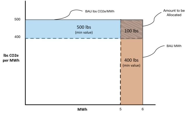
Recall Figure 1 (below) from my last post. It shows that by estimating the avoided emissions from the RPS first (Rate First) would yield 600 pounds of avoided carbon dioxide equivalent (lbs CO2e) (max value) and 400 lbs CO2e for efficiency (min value). The opposite also would be true. So, considering efficiency first (Quantity First) would yield 500 lbs CO2e (max value) and 500 lbs CO2e for the RPS. With this information we have a range of the appropriate value for RPS (500-600 lbs) and for efficiency (400-500 lbs). So, the appropriate value for each is somewhere in its range.

Figure 1 Illustration of Overlapping Emissions between Rate and Quantity Measures

Our proposed method allocates the overlapping emissions reductions based on a weighting factor that represents a measure’s contribution to the overall emissions reduction. So if the RPS yields a higher overall reduction, it would get a higher percentage of the overlapping emissions, and vice versa. Note that a more detailed presentation of this method is included in our recently published article in The Electricity Journal.

We applied this logic to a simple illustrative scenario to consider Governor Brown’s 2030 targets for renewable electricity and efficiency, now codified in SB 350.

Splitting the Baby Method Applied to California’s Energy Policy Targets

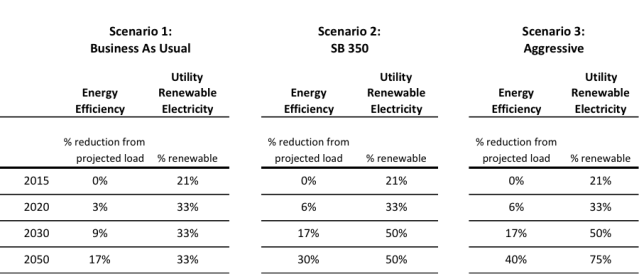
To demonstrate the effects of the Rate-First and Quantity-First methods, and an application of the Splitting the Baby method, we developed three scenarios: business-as-usual (Scenario 1), SB 350 (Scenario 2), and Aggressive (Scenario 3). The business-as-usual scenario assumes that the current RPS requirement of 33% by 2020 is achieved and energy efficiency at forecast levels. The SB 350 scenario increases the RPS requirement to 50% by 2030 and doubles efficiency. Based on the California Energy Commission estimates, this scenario assumes that doubling efficiency in buildings equates to a 17% reduction in projected consumption levels. For simplicity, this efficiency level is applied to all electricity use. The final scenario takes the SB 350 scenario and increases RPS requirements to 75% by 2050 and continues energy efficiency at a slightly slower pace between 2030 and 2050. We applied these targets to the San Diego region to estimate the resulting GHG reductions. Table 2 summarizes the assumptions used through 2050.

Table 1 Assumptions in California State Policy Scenarios

As a reminder, the the results presented here are GHG reductions – it can be counterintuitive to show reductions increasing in a figure. Figure 2 summarizes the results for Scenario 1 – Business-as-Usual. The top cluster of lines shows the emissions reductions associated with rate related changes (RPS), in this case reaching 33% renewable electricity supply by 2020 and continuing at that level through 2050. The top line (blue) represents the emissions reductions when the rate effects are calculated first (Rate-First), the maximum value of the range, and the bottom line (green) is the reductions when the quantity effects are calculated first (Quantity-First), the minimum value. The dashed black line represents the emissions allocated using our method.

Similarly, the bottom cluster of lines shows the emissions reductions associated with quantity related changes (efficiency), in this case reaching 8.5% reduction in electricity use by 2020 and 17% by 2050. The top line (purple) represents the emissions reductions when the quantity effects are calculated first (Quantity-First), the maximum value of the range, and the bottom line (orange) shows the reductions when the rate effects are calculated first (Rate-First), the minimum value. The dashed gray line represents the emissions allocated using the approach presented above.

Figure 2 Results from Business-as-Usual Scenario

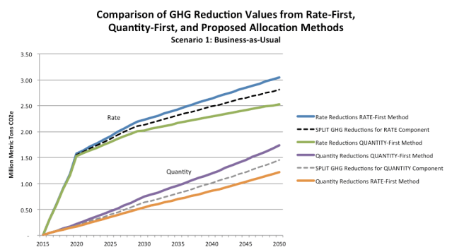
We can make several observations from the results. First, the range between the two different calculation methods increases over time. The difference between the two approaches hardly matters in 2020 but becomes more pronounced by 2050 to about 0.5 MMT CO₂e. For the rate measure, the upper value of the range is 20% higher than the lower value in 2050. For quantity measures, it is 43% higher. Second, the difference between the upper and lower lines for each approach is equal. Third, given the assumptions in this scenario, the split emissions (dashed line) are just below or above the middle of the range. For the rate measures it is just over the middle of the range and the quantity measures is just under the middle. This is because the rate-related measures results in a higher contribution to the overall emissions reduction, therefore, increasing the overall reductions due to the rate-related measure. On the other hand, the quantity measure has a smaller contribution, therefore, decreasing the overall reductions due to the quantity-related measure.

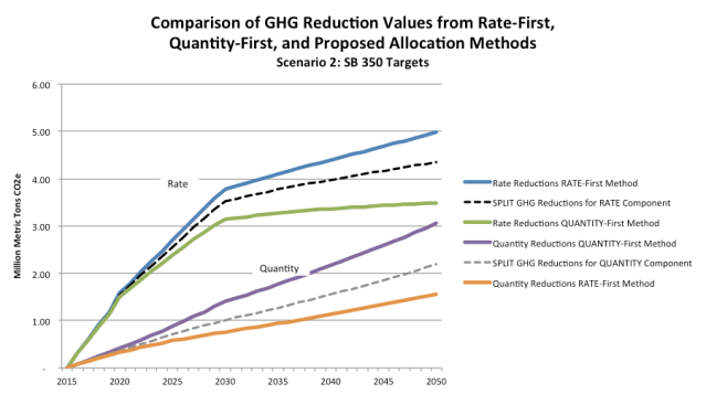
In Scenario 2, the range of emissions reductions between two approaches further widens to about 1.5 MMT CO₂e by 2050 and the split value (dashed line) is higher in the range for the rate measure and lower in the range for the quantity measure (Figure 3). This follows the general concept of the proposed allocation method: the policy that contributes more to the combined reduction gets a higher allocation of the overlapping emissions reductions. The upper range value for rate measures is 43% higher than the minimum value in the range and for quantity measures, the difference is 96%.

Figure 3 Results from SB 350 Scenario

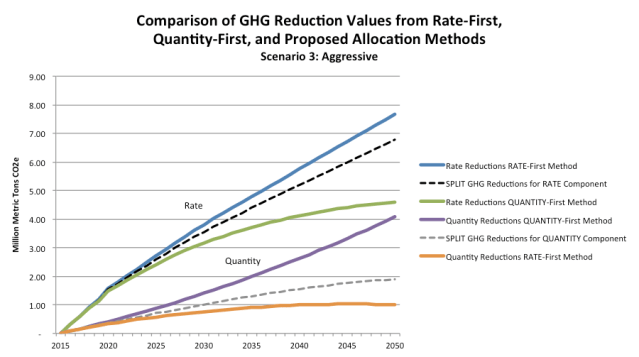
The trends between Scenario 1 and 2 continue in Scenario 3. The overall range by 2050 is over 3 MMT CO2_e and the split value is closer to the maximum value for the rate-related values and closer to the minimum value for the quantity-related values (Figure 4).

Figure 4 Results from the Aggressive Scenario

Mixing and Matching Results from Rate-First and Quantity-First Methods

The differing results illustrate the need for careful consideration in estimating and projecting emissions reductions from policies. If care is not taken, perverse outcomes could result (Figure 5). For example, if two high estimates are combined the total can be significantly higher than the actual value calculated, which is a combination of the Low and High values (Low-High, High-Low).

Figure 5 Combinations of Results

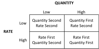
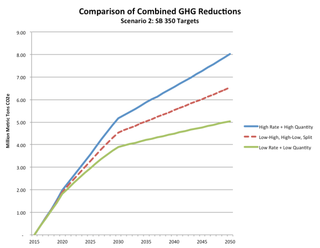
Figure 6 shows the range of the combination of High Rate and High Quantity values, those from Low Rate and Low Quantity values, and the actual values calculated, which are a combination of the Low and High values (Low-High, High-Low). The potential range by 2050 is about 3 MMT CO2e. It is not clear whether this would happen in actual GHG estimates but the possibility exists to overstate the savings in cases where this value is desirable. The opposite also could be true.

Figure 6 Possible Combinations of Results

Policy Implications

The methods discussed here have implications across a wide range of policy and regulatory contexts, including scenario planning to explore combinations of policies to reach targets at any level of analysis (e.g., national, state, local, enterprise) and regulations for which both efficiency and renewable energy improvements are compliance options. This issue is particularly important when estimating the emissions impact from particular mitigation policies or actions. From the U.S. Environmental Protection Agency’s proposed Clean Power Plan to California estimating the impacts of the ambitious goals includes in SB 350 to cities developing climate action plans to new projects demonstrating compliance under the California Environmental Quality Act (CEQA), analytical methods are needed to estimate the impact of policies to reduce greenhouse gas emissions. Absent accepted methods and protocols for calculating GHG reductions, there is room for error that policymakers and regulators should be aware of.