One area of our work at EPIC is to provide technical support to cities, counties, and regional planning organizations in the climate planning process. This work includes estimating greenhouse gas emissions for inventories and the reductions expected from a variety of policies for climate action plans, typically in support of a climate action plan. Over the years our approach to this work has evolved to accommodate methodological challenges that arise, particularly those related to estimated the greenhouse gas reductions that may result from policy. This has gotten us thinking about the critical role methodology plays in the climate planning arena and how it may apply to estimating the future effects of Governor Brown’s climate policy targets and complying with federal policies like the U.S. EPA’s Clean Power Plan.

This is the second post in an occasional series that will discuss methodological issues that arise when quantifying greenhouse gas emissions. My colleague Nilmini Silva-Send recently authored a post that discussed how consumers of greenhouse gas estimates need to be careful to understand what they are getting, in particular the meaning and implications of “business-as-usual.”

The Challenge

This post focuses on the analytical challenge of allocating emissions reductions between policies that affect the quantity of an emitting activity like electricity consumption (e.g., efficiency) and those that affect the rate of emissions of that activity (e.g., renewable portfolio standard). The challenge is that the effects of one policy potentially affect the reductions of the other. In the process of calculating the net emissions reductions from an interconnected suite of policies, it can be necessary to choose the order in which to calculate the impacts of some policies before the impacts of others; the ordering decision affects the magnitude of the emissions reductions for each policy. We wrote about this issue briefly in a previous blog post, which referenced an EPIC Technical Working Paper. We recently published an article on this same topic.

A common method for measuring the level of greenhouse gas emissions is to multiply the total level or quantity of a particular activity by a rate of emissions – or emissions factor – associated with the activity. For example, to estimate the emissions from electricity for a given period one can multiply the total consumption (MWh) in that period by the average electric emissions factor (lbs CO₂e/MWh) in that same period. This method is pretty straightforward.

The same approach if often used to estimate the level of emissions reductions that would result from policies to lower electricity consumption. This is where it gets interesting. While this method may be simple and efficient for measuring total greenhouse gas emissions as in an inventory, it has limitations when used to estimate the emissions reductions associated with a particular policy or activity. One challenge is the order in which the emissions reduction effects of policies are calculated. For example, considering the effects of the renewable portfolio standard (RPS) first would lower the emissions factor and affect all subsequent emissions of other policies such as energy efficiency. That is, the net emissions effect of an energy efficiency measure would be calculated based on a lower emission rate since the RPS has already been accounted for prior to the efficiency measure. The result would overestimate the emissions reduction from RPS and underestimate those from the energy efficiency measure. If the calculation order is reversed, then the opposite outcome arises: reductions from energy efficiency would be overestimated and those from the RPS would be underestimated. The total combined reduction for the two measures will be the same regardless of the order, but the amount allocated to each policy measure will be skewed by the order in which it was calculated.(Note that for our purposes here, we use an average annual emissions factor for electricity but will discuss the role of marginal emissions factors in a future post.)

An Illustrative Example

An example to illustrate this dilemma is helpful. For the purposes of illustration, let’s assume the following:

• The business-as-usual electricity emissions factor before considering the effects of policies like the RPS is 700 pounds of carbon-dioxide equivalent per megawatt-hour (lbs CO₂e/MWh);
• the RPS reduces the business-as-usual electricity emissions rate by 100 lbs CO₂e/MWh;
• the business-as-usual annual quantity of electricity consumption is 6 MWh, and,
• as a result of energy efficiency, annual electricity consumption is reduced by 1 MWh.

There are two ways to estimate the effects of the RPS and efficiency in this case: calculating the effects of the RPS first and then those of efficiency (we call this the rate-first method) and calculating the effects of efficiency first and then those of the RPS (we call this the quantity-fist method). The total reduction of both policies is the same but for both approaches but the allocation between the two policies differs.

Using the rate-first method would account for the effects of the RPS (100 lbsCO₂e/MWh reduction) first and apply it to the entire business-as-usual energy consumption value (6 MWH). Effectively this approach isolates the effect of the RPS by calculating the total emissions before the RPS and then after the RPS and taking the difference as the emissions reductions associated with the RPS. It would overestimate the effects of the RPS (blue) and underestimate the effects of efficiency (orange), since the efficiency reduction would be calculated using the reduces emissions factor (post RPS). The figure below illustrates this effect. In effect this approach would produce a maximum value for the effects of the RPS and a minimum value for the effects of efficiency.

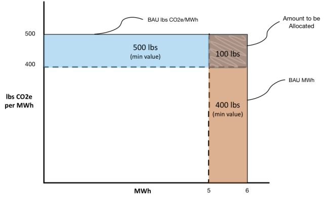
Using the quantity first method would account for the effects of efficiency (1 MWh reduction) first and apply the business-as-usual emissions factor for electricity before the effect of the RPS is applied (500 lbs/MWh). Similarly, this approach attempts to isolate the effect of efficiency by calculating the total emissions before efficiency is taken into consideration using the higher emissions factor and then after the effects of efficiency and taking the difference as the emissions reductions associated with the efficiency. This would overestimate the role of efficiency (orange) an underestimate the role of the RPS (blue). The figure below illustrates this effect. Similarly, this approach would produce a maximum value for the effects of efficiency and a minimum for the effects of the RPS.

So, the allocation of emissions between the RPS and efficiency lies somewhere in between the results of these two methods – between the max and min values for each policy. The following figure illustrates that in both cases the upper right-hand portion of the chart is claimed. This overlapping portion of emissions claimed by each method represents the amount of emissions to be allocated between RPS and efficiency.

The table below highlights the possible outcomes that could result by  mixing and matching the different reduction values. For example, if both minimum values were used, the combined reduction would be 900 pounds. If both maximum values were used, the combined reduction would be 1,100 pounds. The combination of maximum and minimum values gives us the correct amount of 1,000 pounds in this case. 

The question remains, how to allocate the 100 pounds of overlapping reductions? In next post in our greenhouse gas methodology series, I will present a method to distribute or “split” — hence the blog title — the quantity of overlapping emission reductions between the rate and quantity policies.