

Part of understanding climate action plan (CAP) cost analyses results includes identifying what is not incorporated into the analyses. CAP implementation cost analyses (ICAs) and benefit-cost analyses (BCAs) described in earlier posts have inherent limitations that can create a level of uncertainty. This post concludes our CAP cost analyses series by identifying key limitations as they relate to: data availability, benefit and cost ranges, scope of the analysis, timeframes considered, and GHG methodologies.
Data Availability
Estimates for current and future costs and benefits are limited to the data presently available. For some measures, such as a solar PV measure, extensive datasets exist with historic costs associated with installation and operation that can be applied at a local level. However, not all measures have readily available data. For instance, commercial zero net energy (ZNE) construction projects are relatively new in the marketplace and the costs can vary widely depending on the type of commercial project. Case studies reported in the literature can be used, as they are representative of the best available data; however, they may not be entirely reflective of current and/or future conditions.
Additionally, costs and benefits associated with CAP measures are subject to changes in future conditions, such as:
- Population growth and demands;
- Technological advancements and available technology;
- Energy/fuel availability;
- Residential and commercial development stock; and
- Trends in consumer demands and producer supply.
Ranges
The costs and benefits associated with CAP measures can vary across a range of possibilities. For instance, the purchase price of a solar PV system will not be the same for each homeowner, but will generally fall within a range of costs. Ideally, CAP cost analyses could develop high and low estimates in addition to averages (or most likely estimates) to better represent the range in potential outcomes faced (Figure 1). The challenge lies in identifying sufficient data to calculate accurate ranges for all measures and variables included in a CAP. Developing high and low estimates using only select variables can create inconsistencies in results across measures and would misrepresent the true high and/or low estimate impact. As better and more complete data sets become available, it could be possible to develop ranges.
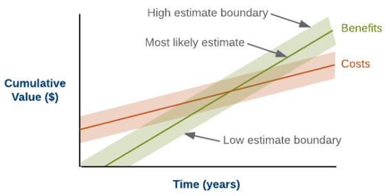
Figure 1. Conceptual Diagram of Benefit and Cost Ranges
Scope
ICAs and BCAs both need to have defined scopes to determine the level of detail to include in the analysis. For an ICA, the scope determines the level of detail to include in the analysis. For a BCA, the scope determines the extent to which benefits and costs associated with a measure are included in the analysis. In both instances, the time and resources available to gather and analyze the necessary data can define the scope.
In an ICA, the scope defines expenditure categories and cost characteristics included in the analysis. For example, an analysis may only estimate staffing impacts and not examine any other expenditure categories. While staffing impacts are necessary to determine CAP implementation costs, it is insufficient to determine the total implementation cost, which could also include costs for capital, consultants, and supplies and materials. Additionally, if a cost estimate focused only on total costs, it would not provide information on the incremental nature of costs.
In a BCA, the scope determines if a benefit or cost is included or not. In general, these analyses capture direct benefits and costs and externalities experienced within a jurisdiction. However, there are other, indirect benefits and costs that can accrue as a result of implementing a CAP. For instance, the production and disposal of materials (e.g., solar PV panels and hybrid vehicle batteries) can have a suite of costs and benefits associated with them. This can include:
- Financial gain by manufacturers;
- Increase in jobs;
- Pollution externalities from hazardous waste disposal at end of useful life; and
- Reduction in pollution caused by traditional energy production (e.g., coal).
Timeframe
Two key parameters in cost analyses related to the timeframe analyzed can contribute to limitations: the baseline year and target year(s).
Baseline Year
BCA calculations incorporate historic data where applicable to account for past activity that leads to GHG reductions in a target year (e.g., 2020). For example, if a CAP has a baseline year of 2010, all related GHG reduction activity between 2010 and the CAP’s target year(s) would be considered to calculate the $/MT CO2e for their respective measures. It is important to note that historic activity would have occurred prior to CAP adoption and is thus not an impact on the jurisdiction or its residents and businesses as a direct result of the CAP. Past activity incorporated into an analysis can under or overestimate the impact of post-CAP adoption activity as prices, rebates, and other variables change over time.
Additionally, the baseline year selected will determine the amount of discounting that occurs by the target year, which influences the present value in a particular year. CAP activity analyzed in 2020 will be discounted back ten years with a baseline year of 2010, but only five years if the baseline year is 2015.
Target Year(s)
Any analysis that involves future projections has some level of uncertainty, which typically increases the further out into the future the projection goes (Figure 2). To reduce uncertainty associated with projections made further out, the cost analyses can be restricted to a near-term target year (e.g., 2020 instead of 2035). As an example, a solar PV system measure has a useful life of 25 years. Evaluating installations in a target year of 2020 would require future projections that extend to 2045 to capture the benefits and costs of that measure. If 2035 is selected as the target year for the BCA, projections would need to extend to 2060. For measures with even longer useful lives, this would require extending projections even further into the future, significantly increasing the uncertainty associated with the results.

Figure 2. Illustrative Example of Increasing Uncertainty with Future Projections
GHG Methodologies
The cost-effectiveness of CAP measures ($/MT CO2e) pairs benefit and cost data with GHG reductions. The order in which reductions are calculated in the CAP for inter-related measures will impact the GHG reductions attributed to each measure and, consequently, the cost-effectiveness ($/MT CO2e) for each measure. An example of interrelated measures include an energy efficiency retrofit measure (reduces electricity consumption) paired with a solar PV measure (reduces emission factor). If GHG reduction estimates are lowered for a measure, the benefit or cost per metric ton will be magnified; if increased, the benefit or cost per metric ton will be reduced. This relationship can be especially challenging when comparing results of similar CAP measures; while reduction calculations within a CAP are consistent, calculations across multiple CAPs may not be.
Wrapping it up
This was the sixth and final post in a series about CAP cost analyses. Earlier posts discussed:
- Part 1: the goals and overall blueprint EPIC has developed for CAP cost analyses
- Part 2: implementation cost analyses (budgetary impacts to the jurisdiction)
- Part 3: benefit-cost analyses framework for CAP measures
- Part 4: cost-effectiveness of CAP measures
- Part 5: impacts of CAP measures on participants
EPIC has applied the concepts discussed throughout the series in analyses for several jurisdictions in the San Diego region, including County of San Diego and City of La Mesa.
For further details on CAP cost analyses, reach out to EPIC director Scott Anders, or me, Marc Steele.
